remaking echo 1 - implementation
this is a follow-up to an earlier article I made about Physical Optics and radar cross sections. In this post, I go through recreating these equations into code and hopefully having enough funny visuals to keep you awake. the first part had an unexpectedly warm reception, big ups to all who actually took the time to read it!
quick recap
RCS (radar cross section) describes the equivalent area that would reflect the same amount of radar energy back to a source. A target with an RCS of 1 m² reflects the same amount of energy as an ideal 1 m² metal plate would12. This is given by the formula
which just describes the ratio of scattered radio to incident radio, while accounting for how waves spread through space in a sphere of size . To optimize a shape, we need to predict its RCS. We use PO, which makes several simplifications to use border cases of Maxwell's equations.
Physical Optics
Recall that according to PO theory, the surface current density on a perfectly conducting surface23 is given by
where is the surface normal and is the magnetic field of the incoming wave. Intuitively, the incoming wave induces currents on the metal surface – think of it like the radar wave “shaking” electrons on the surface – and those moving charges emit the scattered field. The formula comes from enforcing that the tangential electric field on the surface is zero (perfect conductor condition), effectively doubling the incident field as it reflects.
takes a cross on H, the purple arrows reflect the incident field perpendicular to the facet (triangle)
Once we have the surface currents, we integrate over them to get our cumulative scattered field emitted by the whole object:
where represents illuminated surface areas. This integral gives us the scattered field in the direction of the radar. If it looks daunting, the first article might be worth refreshing on.
From math to code
We have the equations, now we have to translate them into code! To begin with, we need some geometry. In a more realistic scenario, you would start with the shape of an aircraft, constrain some points based on what you can't change (engines, etc), and optimize that. For now, we will be using a sphere.
Say hello to sphere.
humble sphere
click to load interactive visualization
You might notice something about sphere. If you look closely, he is uncharacteristically faceted, tiled by triangles. This is because sphere is an icosphere, subdivided by triangle meshes.
It is common practice for meshes to be approximated by triangles4, because they are the simplest shape that can span an area and are guaranteed to lie flat. We could use a function, say
to form an analytic/parametric representation of our 3D object, but it would be painful to work with if we wanted to make any changes other than the radius. If we just make our "sphere" out of triangles, we have subdivisions of points that we can now represent arbitrary shapes with.
Now we can begin actually calculating the RCS of the object! If you recall from part 1, this process is roughly:
- Identify illuminated facets
- Calculate surface currents
- Compute phase
- Sum contributions
As the radar wave passes through the object, represents the surface current induced and the color of the illuminated faces represents the phase
But wait -- our original integral (1) above assumes a continuous function like (2) to sum over the surface. So instead, we have to approximate the integral into a discrete sum5, and go over the triangular faces that make up the surface instead.
If we put these steps into code, it looks something like this:
# Loop over faces
for i in range(len(face_centers)):
    # Check if face is illuminated
    cos_theta_i = np.dot(-ki_hat, face_normals[i])

    if cos_theta_i > 0:  # Face is illuminated
        # Calculate surface current (2n × Hi = 2n × (ki × Ei)/η)
        Hi = np.cross(ki_hat, Ei_hat) / self.eta
        Js = 2 * np.cross(face_normals[i], Hi)

        # Phase at face center
        r = face_centers[i]
        phase = self.k * (np.dot(ki_hat, r) - np.dot(ks_hat, r))

        # Contribution to scattered field
        # Es ~ (ks × (ks × Js)) * exp(jkr·(ki-ks)) * Area
        ks_cross_Js = np.cross(ks_hat, Js)
        integrand = np.cross(ks_hat, ks_cross_Js)

        # Project onto receiving polarization
        contribution = np.dot(Es_hat, integrand) * face_areas[i] * np.exp(1j * phase)

        scattered_field += contribution
JAX speedups
This is great, but looping through faces is inefficient. Thanks to the power of modern computing, we can make this process embarassingly parallel, and calculate the scattered field for the whole object at once!
# Face illumination mask
cos_theta_i = face_normals.dot(-ki_hat)
illuminated = cos_theta_i > 0

# Surface currents (constant Hi, Js varies with normals)
Hi = np.cross(ki_hat, Ei_hat) / self.eta  # (3,)


Js = 2 * np.cross(face_normals, Hi)  # (N,3)
Js[~illuminated] = 0.0  # Mask non-illuminated faces


# Phase term for each face
phase = self.k * (
    face_centers.dot(ki_hat) - face_centers.dot(ks_hat)
)
phase[~illuminated] = 0.0


# Scattered field integrand
ks_cross_Js = np.cross(ks_hat, Js)  # (N,3)
integrand = np.cross(ks_hat, ks_cross_Js)  # (N,3)


# Projection onto receiving polarization and aggregation
proj = integrand.dot(Es_hat)  # (N,)
proj[~illuminated] = 0.0


contributions = proj * face_areas * np.exp(1j * phase)
scattered_field = contributions.sum()
scattered_field *= (self.k / (2 * np.pi))

# Calculate RCS: σ = 4π|Es|²/|Ei|²
# For far field, |Ei|² = 1 (normalized)
rcs = 4 * np.pi * np.abs(scattered_field)**2
Designing a shape
Now that we have a way to compute RCS, how do we use this to create an optimized shape? This is actually a pretty interesting question, and there's a number of ways you could do this.
Manually
Echo 1 predates modern optimization methods; engineers back then would actually manually tweak the shape fed into the program, with the designers themselves being the feedback loop. They would change the shape a little, see how the RCS changed, then use their intution to build the next model to feed in again.
"There were no computers. Everything was done manually. We had guys carving shapes out of balsa wood to test their radar reflections. For Echo 1, we didn’t have the math or the modeling tools. So we relied on physical intuition and endless trial-and-error in the RCS range." — Ben Rich6
We don't want to do this. I am neither as smart nor as patient as those Skunkworks engineers, and I would like my computer to do this for me. If we want to optimize our shape numerically though, we're gonna need a medium for it to make changes through.
Deformation Vectors
A simple approach is for the program to take points on the mesh and generate deformation vectors that then tell it how to move the shape:
We then take the RCS of this, and repeat using our chosen optimization method to generate new deformation vectors, until we reach a minimum. We can imagine this as having a clay ball, and an iterative process of saying how to "mold" the ball in order to minimize its RCS. This analogy also hints at a key weakness of this method.
If you only generate deformation vectors to "squeeze" your shape into a more optimal one, what if your optimal shape contains many holes? You're only moving points that already exist smoothly, so you're limited to the initial topology you fed in. You can't create or remove holes, because in a topological sense, all you're doing is applying a continuous transformation to the surface, and your mesh's connectivity remains static. This is similar to the famous example of a coffee cup being equal to a donut; you can only have as many holes as you start with.
However, when designing a plane, you rarely want to spontaneously create holes, so this smooth transformation is actually somewhat ideal under our constraints -- imagine just putting in a wing and wanting to elongate/angle it. However, there are other methods to work around this limitation
Density-Based Methods
A density-based method treats the material as a grid of voxels, where each element can either be a 0 or 1 depending on if material should exist. Then, the optimizer can effectively delete or add regions to suit the topology to change. This is true optimization over the material distribution, instead of deforming the geometry, and allows the program to make all the holes it would like7
This comes with some tradeoffs though; in return for a better global optimum, you now need to filter the shapes so it can't cheat by making physically valid structures. By giving free reign over the shape, you allow a myriad of unmanufacturable things to be optimized. This is doable, but outside the scope of my project
Optimizers
Now that we have an objective function (RCS calculation) and a way to play with a mesh (Deformation vectors), we need a way to continuously generate such that is minimized.
Being from an ML background, my immediate thought was to use Adam.
Adam!
Adam8 is a momentum-based gradient-descent algorithm. Explaining gradient descent is somewhat outside the scope of this article, but 3b1b has an excellent video that describes the specifics.
Adam (purple) vs Gradient Descent (orange): Adam finds global minimum easier due to momentum
In this visual, you can imagine each ball representing a candidate set of deformation vectors. The surface they "roll" on is the loss plane, which is the calculated gradient of our RCS loss. To reach the lowest RCS, we need to reach the global minimum -- the well in the center -- to find our most promising deformation vectors, which then gives us our optimal shape.
The orange ball performs standard gradient descent, and it gets stuck in a local minimum. Adam, represented by the purple ball, adds some momentum to be ball, making it easier to overcome small perturbations to reach a lower global minimum faster.
Even though Adam has momentum, if our hill is steep enough, we can still get stuck in a local valley.
Differential Evolution (DE)
What if, instead of hedging our bets on one ball, we just start with multiple and see which one hits the bottom? More importantly, what if our gradient is rife with mountains and valleys? Gradient descent wants to go towards minimizing the objective function, but what if the objective function is not very predictable? This is often the case in a topological problem like this one, where a certain feature can change the characteristics of the shape entirely. This is where DE9 comes in.
Instead of traversing the gradient, we can store sets of candidate deformation vectors, and, just like a Genetic Algorithm, we mimic evolution and "breed" successful vectors by interpolating them.
So:
- Create a population of deformation vectors, , and calculate their RCS .
- Define a fitness function based on RCS and constraints like smoothness or volume preservation by applying a smoothness or volume penalty for example:
Now, for each generation:
-
Mutation: For each individual , pick three distinct individuals , , from the population (where ), and generate a mutant vector :
where is the differential weight controlling amplification of the differential variation.
-
Crossover: To add genetic diversity, we mix the parent and the mutant to get a trial vector using binomial crossover:
where is the crossover probability, and is a randomly chosen index to ensure at least one element comes from the mutant.
-
Selection: The new vector replaces the old one only if it improves the fitness:
Repeat this for a number of generations or until convergence. In code, this translates to something like
# Mutation: pick 3 random individuals and create mutant
indices = jax.random.choice(key, pop_size, (3,), replace=False)
indices = jnp.where(indices == i, (indices + 1) % pop_size, indices)  # ensure distinct
mutant = population[indices[0]] + F * (population[indices[1]] - population[indices[2]])
# Crossover: mix mutant and original
cross_mask = jax.random.uniform(key, (n_dims,)) < C_r
j_rand = jax.random.randint(key, (), 0, n_dims)  # guarantee at least one gene from mutant
cross_mask = cross_mask.at[j_rand].set(True)
trial = jnp.where(cross_mask, mutant, population[i])
This is more computationally challenging per iteration, but allows for more exploration of the space, more of a "trial by error" approach.
Confirmation
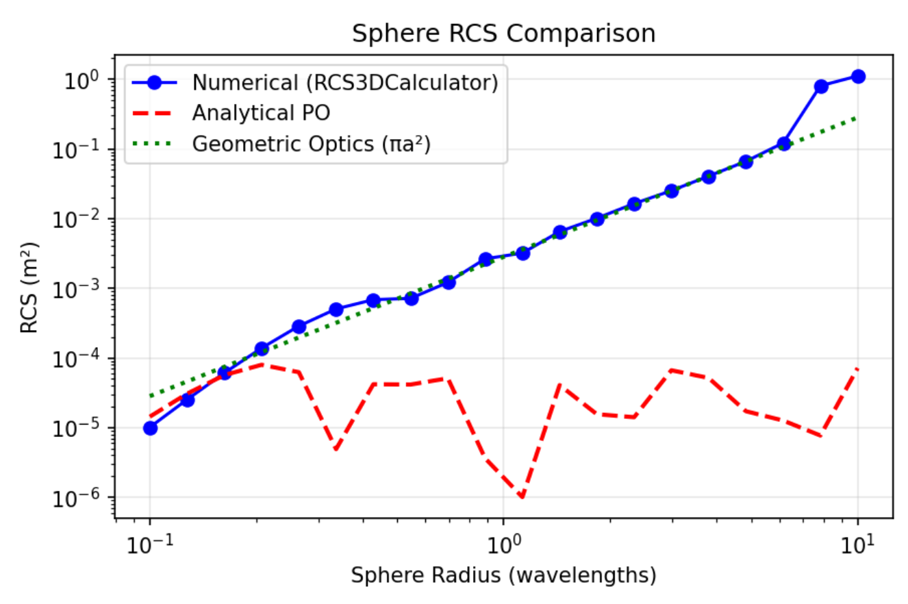
Now that we have our optimizer, to make sure it's working somewhat as expected, let's run some calcs to compare it to the Mie solution 10 to see if we're close.
 1753251688985_vo6nj4.png
Our solution (Analytical PO) seems to be a lot lower than expected, and has somewhat irregular valleys/mountains. Why is this?
For a long time, I struggled to figure this out, assuming there was some errors in my calculations. There were, but even after I tried every permutation of confirming the math, this depression persisted.
creepy waves
What I had stumbled onto was one of the core weaknesses of PO. Recall that one of the assumptions we make is that only illuminated faces contribute surface current to the scattered field. It turns out, for curved objects, a significant portion of the radar returns are generated by "creeping waves"1112 -- radar that travels along the curve and produces backscatter towards the source. To illustrate this a little better, I made a short animation:
Curves provide a medium for these waves to creep along, so a sphere was in many ways a cas study for this weakness of PO. Another somewhat surprising thing is that the RCS signature for a faceted sphere (like the one we're optimizing here) is actually quite spiky. This feels wrong, but if you !imagine a disco ball and think of how often light will "glint" back at you, it makes more sense.
sphere rcs
click to load interactive visualization
a sphere's radio signature is quite spiky when it's faceted!
On the other hand, PO also ignores the fact that diffracted edge currents can destructively interfere1213. This isn't that big of a concern on a sphere, but becomes more apparent on faceted surfaces like aircraft geometry. Thus, PO tends to underestimate the RCS for heavily curved objects, and overestimages faceted geometry.
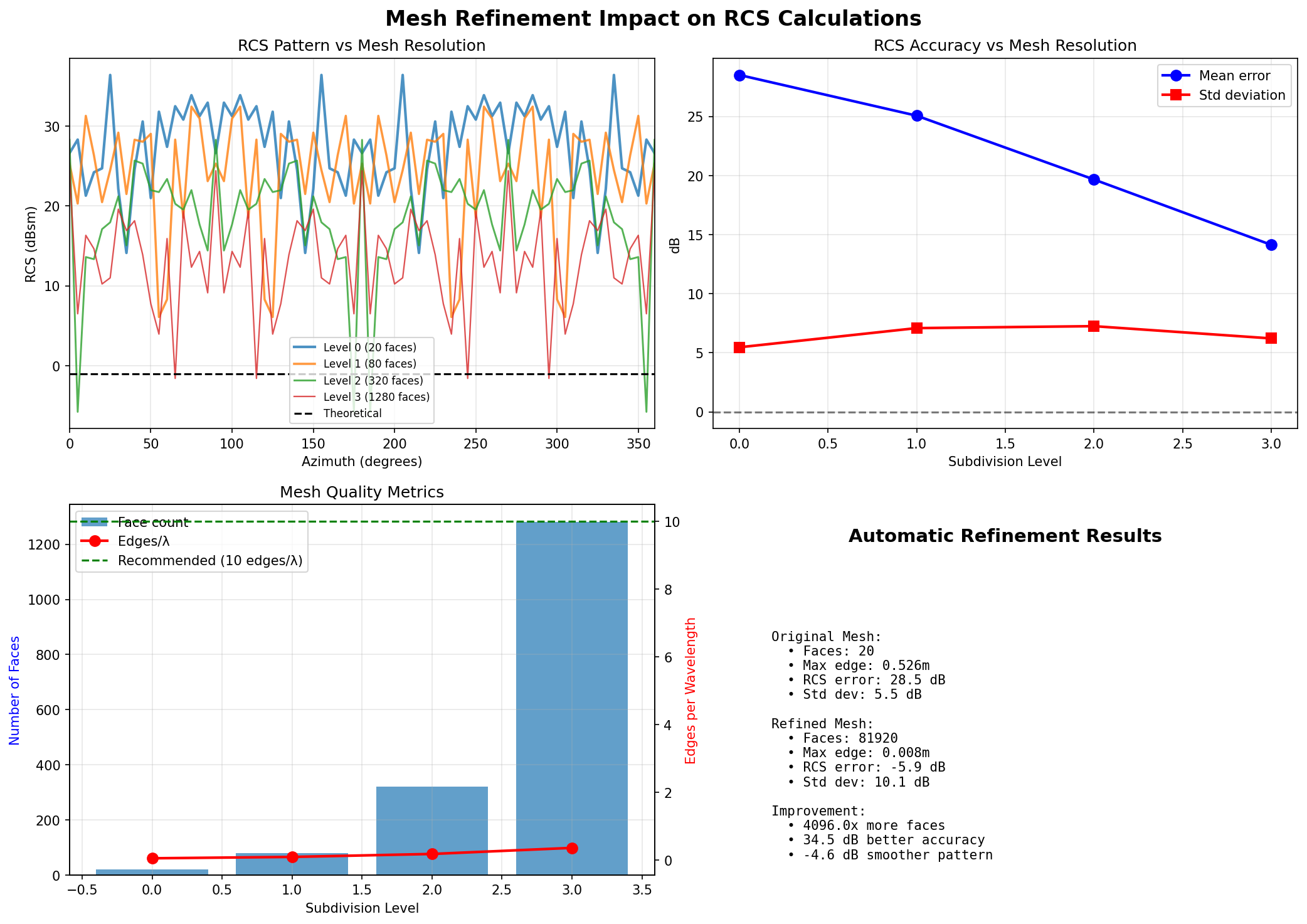 1753257958936_lr7yw3.png
In general, increasing the mesh density increases the accuracy of our calculations as well. This reduces the "spikiness" caused by having facets instead of a continuous surface, better approximating the integral in eq (1) from earlier3.
1753257958936_lr7yw3.png
In general, increasing the mesh density increases the accuracy of our calculations as well. This reduces the "spikiness" caused by having facets instead of a continuous surface, better approximating the integral in eq (1) from earlier3.
When I compared my calculations' values to flat plates and faceted surfaces, I returned to perfect ground truth. It turns out that a sphere is somewhat of a psychotic edge case to test this method on. oh well.
stealthy sphere
Now that we've verified calculations and set up every piece of the puzzle, we can start optimizing. To recap we're
- Calculating the RCS of our starting shape
- applying a deformation as determined by Differential Evolution
- recalculating the RCS, then moving on to the next generation
until our loss stops going down or we hit a certain number of generations! Now, to have something to optimize towards, we're going to need to define some radar points.
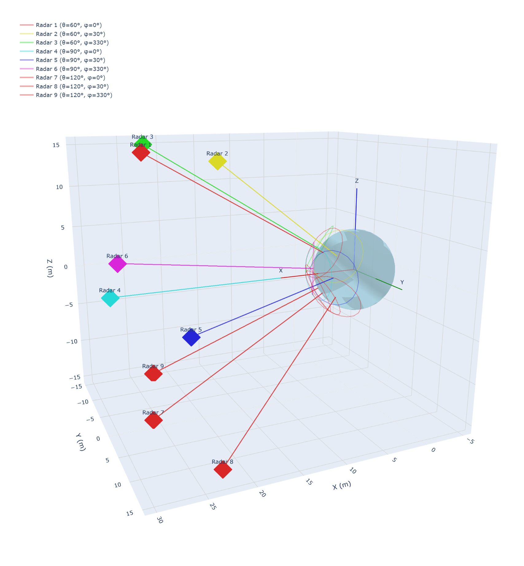 1753282419504_0tgne7.png
Now, we just run our optimization!
1753282512420 zt4fai
click to load interactive visualization
As hoped, we can see that the sphere starts to develop facets as it tries to minimize its radar cross section. In this example, the volume constraint is on, so the program can't cheat by making itself smaller, and there's alsso a smoothness constraint so it can't make sudden changes to the topology. It's interesting to note that if we take these off, we get something like this!
1753282997741 i9o0os
click to load interactive visualization
With no restrictions, the optimizer "crumbles" the ball in order to brute-force a lower RCS!
say goodbye to sphere
Now that we've confirmed that we have a pipeline that works, it's time to optimize something more airplane-like. something more faceted, and less troublesome.
I'll create a baseline "plane." His name is Thud, an onomatopoeia for his flight career should it (or he) ever arise.
thud
click to load interactive visualization
Okay, he is not the prettiest plane on the block. But you should give me a break, because he looks like this:
# Top pyramid vertices
vertices = [
    # Nose point
    [15.0,  0.0,  0.0],
    # Front top edges
    [10.0, -3.0,  2.0],
    [10.0,  3.0,  2.0],
    # Wing leading edges
    [ 0.0,-12.0,  0.5],
    [ 0.0, 12.0,  0.5],
    # Rear top points
    [-10.0, -8.0, 0.0],
    [-10.0,  8.0, 0.0],
    [-12.0,  0.0, 1.0],
    # Bottom vertices (mirrored lower Z)
    [10.0, -3.0, -1.0],
    [10.0,  3.0, -1.0],
    ...
]
To stay true to the history, I hand-tuned a plane-like structure, just as early stealth designers did. Though I, unfortunately, am privy to seeing how bad it looks on a screen, rather than on paper. Now, all have to do to pretend I'm Kelly Johnson is tweak the angles until the cross section decreases! To increase realism slightly, I also added some more radar angles that a stealth aircraft would likely be optimizing for14.
the evolution of thud
click to load interactive visualization
I don't know about you, but that almost looks like it could be a plane!
Obviously I jest, and some more care has to be taken into making this geometry feasible, as well as adding constraints, but foundationally this is it! In a more modern implementation, aerodynamics would usually be added as a secondary objective to the loss function, so the object ends up a little better off than Thud here as well, but I'm more than comfortable stopping here for now.
conclusion
This should help explain how stealth aircraft end up with such bizarre and extreme geometry -- it is literally optimal! This article ended up going in a lot more directions than I anticipated, much like my personal learning journey did. I hope you find it as worthwhile as I did.
Footnotes
-
Skolnik, M. I. (2008). Radar Handbook (3rd ed.). McGraw-Hill. ↩
-
Knott, E. F., Shaeffer, J. F., & Tuley, M. T. (2004). Radar Cross Section (2nd ed.). SciTech Publishing. ↩ ↩2
-
Balanis, C. A. (2012). Advanced Engineering Electromagnetics (2nd ed.). Wiley. ↩ ↩2
-
Botsch, M., Kobbelt, L., Pauly, M., Alliez, P., & Lévy, B. (2010). Polygon Mesh Processing. AK Peters/CRC Press. ↩
-
Harrington, R. F. (1968). Field Computation by Moment Methods. Macmillan. ↩
-
Rich, B., & Janos, L. (1994). Skunk Works: A Personal Memoir of My Years at Lockheed. Little, Brown and Company. ↩
-
Sigmund, O. (1998). “A 99 line topology optimization code written in MATLAB.” Structural and Multidisciplinary Optimization, 21(2), 120–127. ↩
-
Kingma, D. P., & Ba, J. (2015). “Adam: A Method for Stochastic Optimization.” ICLR 2015. ↩
-
Storn, R., & Price, K. (1997). “Differential Evolution – A Simple and Efficient Heuristic for Global Optimization over Continuous Spaces.” Journal of Global Optimization, 11, 341–359. ↩
-
Mie, G. (1908). “Beiträge zur Optik trüber Medien, speziell kolloidaler Metallösungen.” Annalen der Physik, 330(3), 377–445. ↩
-
Keller, J. B. (1962). “Geometrical Theory of Diffraction.” Journal of the Optical Society of America, 52(2), 116–130. ↩
-
Ufimtsev, P. Y. (1971). Method of Edge Waves in the Physical Theory of Diffraction. Foreign Technology Division (U.S. Air Force translation). ↩ ↩2
-
McNamara, D. A., Pistorius, C. W. I., & Malan, J. A. G. (1990). Introduction to the Uniform Geometrical Theory of Diffraction. Artech House. ↩
-
Martins, J. R. R. A., & Lambe, A. B. (2013). “Multidisciplinary Design Optimization: A Survey of Architectures.” AIAA Journal, 51(9), 2049–2075. ↩